Statistical tests for detecting reference product change in biosimilar studies
Published on 2023/05/04
Generics and Biosimilars Initiative Journal (GaBI Journal). 2023;12(2):50-60.
Author byline as per print journal: Jiayin Zheng1, PhD; Peijin Wang`2, MS; Yixin Wang3, PhD; Shein-Chung Chow2, PhD
|
Abstract: |
Submitted: 23 August 2022; Revised: 3 January 2023; Accepted: 12 January 2023; Published online first: 25 January 2023
Introduction
For the approval of biosimilar products, the US Food and Drug Administration (FDA) recommends a stepwise approach for obtaining totality-of-the-evidence in support of regulatory submissions of biosimilar products. The stepwise approach includes assessments of analytical similarity, pharmacokinetic (PK)/pharmacodynamic (PD) similarity, and clinical similarity [1]. For the assessment of analytical similarity, FDA suggested 6–10 lots of the proposed biosimilar (test) product and the innovative (reference) product be tested for critical quality attributes (CQAs), that are relevant to clinical outcomes [2, 3].
For a given CQA, the recommended equivalence acceptance criterion (EAC) of an equivalence is 1.5 σR, where σR is the standard deviation of the reference product. This EAC is proposed based on the following assumptions: (i) a smaller than σR/8 mean difference is allowed for biosimilarity; and (ii) the mean difference is proportional to σR [2]. This equivalence test has been criticized because: (i) the EAC is data dependent; and (ii) the assumptions may not be met in practice. When the population means and variances of the test product and the reference product are similar, use of the method of quality range (QR) is suggested by FDA [3]. However, when the assumption for mean/standard deviation is not held, Son et al. [4] have shown that QR method may lead to approving biosimilar products that are not truly biosimilar.
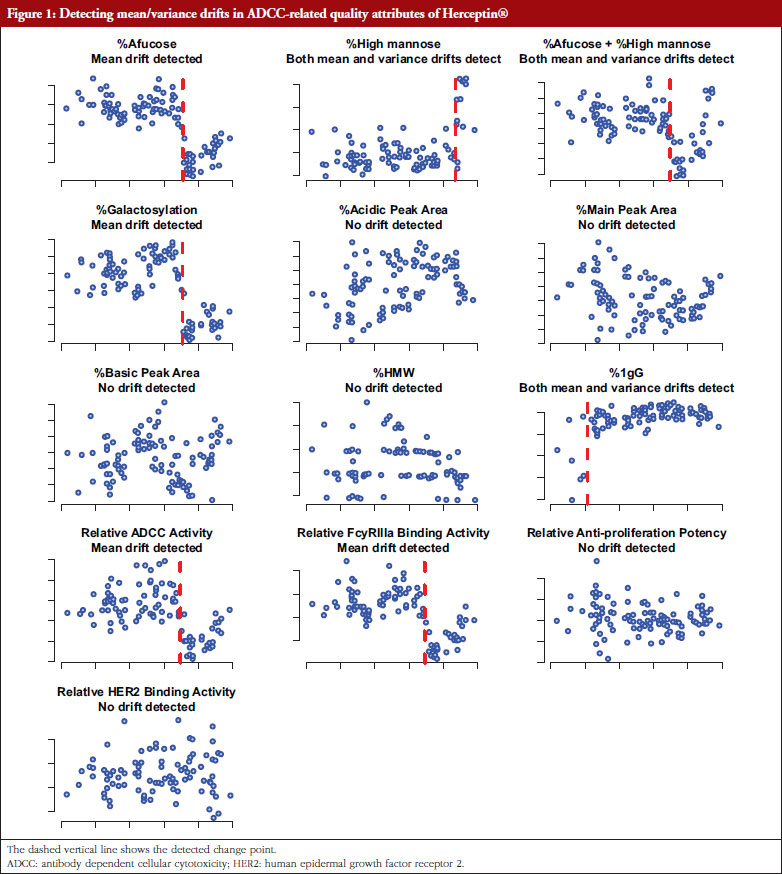
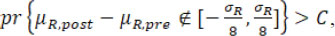
The issue this paper focuses on is that, when performing analytical similarity assessments of certain CQAs that are relevant to clinical outcome, a potential drift in mean response and/or drift in variability associated with the response of the reference product over time may be observed. The drift is defined as an unintended process variation resulting in gradual changes or sudden shift in a quality attribute [5]. Many literature reports revealed drifts exists in biosimilar reference products [6-8]. For example, in the development of Herceptin®, a biosimilar product to trastuzumab, drifts of %afucose and %high mannose were observed [7]. Ramanan & Grampp [8] have shown that darbepoetin alfa (Aranesp®) has the same drift problem found in reference product. Small changes in the manufacturing process of a biosimilar product may lead to great impact on their function [9], therefore avoiding these tiny differences is of great importance. When drift(s) exists in a reference product, it is of interest to determine which lots (i.e. reference lots before the drift, after the drift, or combined) should be used for analytical similarity assessment between the proposed biosimilar product and the reference product. The results of a similarity assessment may depend on the selection of the similarity margin, which is determined based on an estimate of the variability of the test results of selected lots of the reference product. Additionally, the type of drifts may also be of great importance. This in silico study was done to determine how to assess: (i) at what time the drift in mean response and/or drift in variability has occurred; and (ii) which lots should be used for assessment of analytical similarity.
For potential drift in mean response and/or drift in variability, there are three possible scenarios: (i) drift in mean response but no drift in variability; (ii) no drift in mean response but drift in variability; and (iii) drifts in both mean response and variability. For example, as shown in Figure 1, Herceptin® has been found to have mean drifts in %Afucose, %Galactosylation, relative antibody dependent cellular cytotoxicity (ADCC) activity relative FcyRIIIa blinding activity, and both mean and variability drifts in %high mannose and %IgG. For cases: (i); and (ii), a traditional quality control (QC) chart for mean response and variability can be used [10, 11]. In recent years, change point detection methods have been developed aimed at the identification and analysis of complex systems whose underlying state changes, possibly several times [12, 13]. These well-developed change point approaches have shown promising potential in detecting drifts related to all the three scenarios simultaneously, without the need to test specifically each one of the three scenarios.
This article focuses on using adequate change point methods for detecting possible drifts in mean and/or variability of the response of the reference product, under the context of analytical biosimilarity assessment with limited sample size for both the test and reference products. When a change point is detected, use of a fiducial-inference-based method is proposed [14, 15] to test the following hypotheses: (i) whether the difference of pre- and post-change point means falls within an acceptable interval, say (– σR/8, σR/8) where the estimate  is treated as the true σR; (ii) whether the ratio of pre- and post-change point standard deviations falls within a pre-specified interval, say (2/3, 3/2). This statistical test will give more rigorous results compared to using time-ordered trend scatter plot to detect drifts. Extensive simulation was conducted to evaluate the performance of the change point approaches for detecting the drifts, and the proposed fiducial methods for testing the hypotheses regarding mean/variability drifts, under a variety of practical parameter configurations. The detection process is illustrated using an example. Finally, concluding remarks and some practical recommendations based on our simulation findings are provided.
Methods
Notation and data
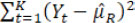
For a given CQA, FDA recommends that a single test of each lot be performed. Without loss of generality, assume that the selected test lots are manufactured (or released) at different times. Let Yt be a test result of the reference lots at time t, with its probability distribution function denoted by F t, where t = 1, …, K. A change point occurs at τ when Fτ ≠ Fτ+1. Depending on the specific application context, it is often assumed that the distributions  belong to a common parametric family or alternatively that they require using a non-parametric setting. For example, in this report it was assumed that Yt is normally distributed with mean µt and a standard deviation σt. Then Fτ ≠ Fτ+1 is equivalent to ( μ t+1, σ t+1) ≠ ( μt+1, σ t+1). In this setting, a drift occurs at , τ if and only if there exists a mean drift indicating that μτ ≠ μτ+1 and/or a variance drift implying that στ ≠ στ+1.
For the sequence data  , the ( b – α)-sample long sub-data
  (0 ≤ a < b ≤ K) is simply denoted by Y a,b. Therefore, the complete sequence data is Y 0, K. We denote a set of indices by a calligraphic letter:
  and as its cardinality. Also, let be the M time points where the drift occurs either in mean response, or in variability associated with the response, or both.
Detection of change points
The task of change point detection involves finding drifts in trends in the underlying model of long and noisy sequence data [16, 17]. It consists of two main branches: online methods that aim to detect changes as soon as they occur in a real-time setting, and offline methods that retrospectively detect changes when all samples are received [12]. The focus of this article, detecting underlying drifts in mean/variability in the sequence data of the reference product, is a proposed solution to an offline change point detection problem. Below offline change point detection approaches are briefly introduced.
Change point detection consists of estimating the indices for potential changes  . Depending on the context, the number M of changes may or may not be known, in which case this also has to be estimated. Generally, change point detection is equivalent to a model selection problem of choosing the best possible segmentation
  according to minimizing a loss function
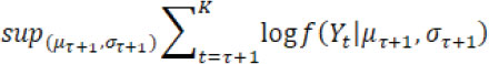
  . The choice of loss function depends on preliminary knowledge and encodes the type of changes that can be detected. For instance, assume Yt follows a normal distribution and consider identification of a single change point, then the loss function can be defined by
for a candidate single change point 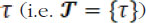 and
and
For no drift (i.e. is empty), where f( Yt| µ ,σ) is the probability density function of a normal distribution with mean µ and variance σ
When the number of changes is unknown, a penalty function () which is an appropriate measure of the complexity of a segmentation , is often added to the loss function and then is minimized to obtain the best segmentation . Popular standard penalty functions used within the change point analysis are, for example, SIC (Schwarz information criterion), BIC (Bayesian information criterion), and AIC (Akaike information criterion).
To solve this optimization problem, different searching methods have been proposed, in an exact fashion or in an approximate fashion. In this article, the PELT/AMOC algorithm [18] is used that applies when the number of changes point is unknown or there is at most one change point, to minimize the penalized loss function + pen. Specifically, an R package ‘change point’ was used to implement the task of detecting drifts in mean/variance of the reference product in the simulation and example [19]. This package provides ways to do detection under the three scenarios: mean drift only, variance drift only, and both.
Note that the drift detection for the reference product in assessing biosimilarity has its own characteristics and that the sequence data size K is often quite limited. Therefore, the detection power could be inadequate for minor drifts, but it is often practically plausible to presume that at most one change point (denoted by t*) occurs in the sequence data.
Hypotheses testing for mean/variability drifts
Consider four underlying scenarios regarding the mean/variability drifts of the reference product:
- No drift in mean and variability
- A drift in mean at t* but no drift in variability
- No drift in mean but a drift in variability at t*
- A drift in both mean and variability at t*
Since the occurrence of the time of the true drifts are unknown, there are two possible procedures for analytical biosimilarity assessment:
Procedure A: Just use the entire data 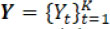 as the reference product sample to estimate the variability σR and subsequently assess biosimilarity µR;
Procedure B: First use appropriate methods to detect potential mean/variability drifts and then use proper reference product sample for biosimilarity assessment. Assume the detected change point is if any, and set  if no drift is detected. Specifically, for the three cases:
(B.1) Detect only mean drift, assuming no variability drift
(B.2) Detect only variability drift, assuming no mean drift
(B.3) Detect any of mean/variability drifts.
Compared to Procedure B, Procedure A is less accurate due to the ignoring of any potential drifts. Hence, in this section, more detailed mathematical derivations about Procedure B are illustrated.
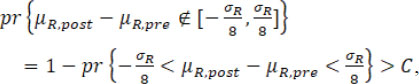
For simplicity and illustration purpose, assume there is at most only one drift in mean/variance. When a change point is detected, it is proposed that to test the following hypotheses regarding mean/variance drifts with the detected change point be treated as fixed. If only drift in mean is detected (as B.1), the following hypotheses are tested:
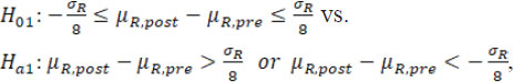
where µR,pre and µR,post are the underlying means of the sequence data before and after , respectively, and the estimate  based on the data Y is treated as the true σ R.
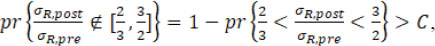
If only drift in variability is detected (as B.2), the following hypotheses are tested:

where σR,pre and σR,post are the underlying standard deviations of the sequence data before and after , respectively. If the drift exists in both mean and variability (as B.3), both hypotheses ( H01 vs H a1 and H02 vs H a1) are tested. Note that here the margin scales of the hypotheses, i.e. σ R/8 and 3/2, are selected such that they are consistent with the margins currently recommended by FDA (FDA, 2017). Alternatively, specific margins can also be selected based on specific practical context and empirical knowledge.
When no change point is detected or the hypotheses are not rejected given a change point detected, using all reference product data in estimating σR and subsequent µR assessment is recommended, since there is no statistically significant drift. When H01 is rejected under B.1 or only H01 is rejected under B.3, the post-change point reference product sample 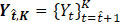 may be used for assessing µR and the entire sample Y may be used for estimating σR. When H02 is rejected under B.2 or only H02 is rejected under B.3, the entire sample Y may be used for assessing µ R and post-change point sample
  may be used to estimate σR. When both H02 and H02 are rejected under B.3, the post-change point sample may be used for both estimating σ R and µ R.
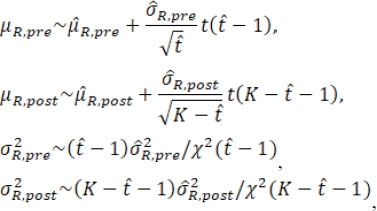
Next, the test to test for H01 and H02 based on fiducial probabilities are illustrated. Here, the detected change point is treated as fixed [13, 14]. Let denote the detected change point, and 1 < < – 1. The pre- and post-change point estimated means and variances are
and the overall mean and variance estimators are
When the estimated is equal to the true change-point t*, these point estimators satisfy
where t( υ) and χ2( υ) are the Student’s t distribution and Chi-square distribution with the degree of freedom υ. Then the fiducial distributions of µR.pre, µR.post, σR.pre, and σR.post are
where the estimates 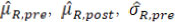 and
and  are now treated as constants. Treating as fixed, the four ‘random’ quantities, µR.pre, µR.post,
  , and
, and  are statistically independent. Denote
 . The fiducial probabilities of similarity in mean/variance between pre- and post-change point reference products are
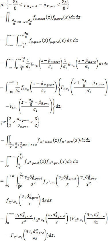
where fµ.post( X), fµ.pre( X), fσ2.post( X) and fσ2.post( X) are the PDFs (probability density functions) of the fiducial distributions of µR.pre, µR.post, and , respectively, with the corresponding CDFs (cumulative distribution functions) Fµ.post( X), Fµ,pre( X), Fσ2,post( X) and Fσ2,pre ( X) respectively; ft,v( X) and Ft,v( X) are the PDF and CDF of t distribution with the degree of freedom v, and f X2, v( X) and F X2, v( X) are the PDF and CDF of the Chi-square distribution with the degree of freedom v. Numerical integration can be used to get an accurate estimation of these fiducial probabilities. Given a pre-specified critical value C, we propose the following testings based on fiducial probabilities.
Under Procedure B.1 for which assuming equal variances across time, the overall variance estimator 
 is inappropriate to serve as the variance estimator for each time point given potential mean drift and alternatively an unbiased weighted version of the estimator can be used

So rather than  is treated as the true σR. If the calculated fiducial probability of dissimilarity in mean is larger than critical value C, i.e.
the conclusion would be that a mean drift occurs at the change point ; otherwise, there is no evidence of a mean drift.
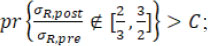
Under Procedure B.2, if the calculated fiducial probability of dissimilarity in variability is larger than C, i.e.
the conclusion is that a variability drift exists at the change point ; otherwise, there is no evidence that a variability drift occurred.
Under Procedure B.3, first the null hypothesis H02 is tested by checking if
then the null hypothesis H01 is tested by checking if
treating as the true σ R.
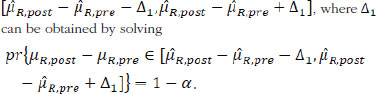
Besides similarity testing, fiducial probability can also be used to construct fiducial intervals. For the mean drift µR,post — µR,pre, 1 – α the arithmetic symmetric fiducial interval is
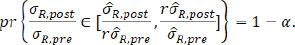
For the variability drift in terms of the ratio of σR,post over σR,pre, the 1 – α geometric symmetric fiducial interval is  , where r can be obtained by solving
These fiducial intervals enjoy the advantage that unlike traditional confidence intervals, this does not impose the assumptions like equal standard errors and thus does not need to make adjustment to accommodate the violation of this assumption. For single mean or standard deviation, like µR,pre, µR,post, σR,pre, or σR,post, the fiducial interval is numerically identical to the confidence interval. For functions of multiple parameters, like µR,post — µR,pre, or σR,post/ σR,pre, they are generally different and the fiducial interval can be easily derived.
Though this hypothesis testing approach can help detect and test for change point(s), it will lead to false positive rate inflation. Specially, the false positive rate inflation exists due to two reasons. The first one is that if there are more than one change points, the hypothesis testing for drifts will be conducted more than once. Hence, the false positive rate will be inflated. Another reason is that in biosimilar studies, drift detection is just the first step, further analyses, such as bioequivalent tests will also be conducted. Then, the false positive rate will increase since the data were already ‘looked at’ in the drift detecting process. Therefore, false positive rate inflation is an issue that needs to be considered. Sequential testing approaches, such as the Holm approach [20], could be used to control for false positive rate inflation.
In practice, the critical value C can be chosen as 0.8 or 0.9, depending on the sample size of the reference product and other context-specific considerations. When a mean/variability drift is detected, the post-change point sample that would be used may be limited by sample size for assessing biosimilarity. Therefore, it is probably necessary to supplement additional samples Y s that are sampled from the same population as the selected post-change point sample , and combine and Y s for assessing biosimilarity in order to avoid power loss.
Simulation study
In this section, extensive simulation studies are conducted to investigate the performance of the proposed methods in detecting the change point and testing the hypotheses of no drift in mean/variance of a reference product.
A variety of parameter configurations are considered. The total sample size of the reference product is chosen as K=20, 60, 100, and 5,000, where the first three are practical choices and last one is a large sample case used to validate the limiting properties of the proposed methods. Assume there is at most one change point. The true change point is at t* = 0.8 × K, if existed. The critical value is set as C = 0.8 or 0.9.
The first half sequence data are generated from normal distribution with mean µ R,1 = 0 and standard deviation σ R,1 = 1; for the second half sequence data, the standard deviation σ R,2 is set to 1/4, 1, or 4, and the mean µ R,2 is set to
where q = 0,1/16, 1/8, 1/4, 1/2, 1 or 2. When σ R,1 = σ R,2 = σR, µ R,2 is simply qσR. For those parameter configurations, there are 7 × 3 × 4 × 2 = 168 scenarios in total. The simulation is conducted with 1,000 iterations.
For each of the 168 simulation scenarios, four rejection rates are reported for the combined process that first detecting change point and then testing the hypotheses of no mean/variance drift under different procedures: test H01 by Procedure B.1, test H02 by Procedure B.2, test H01 and H02by Procedure B.3.
Table 1 shows these rejection rates under each scenario. When the sample size is large ( K = 5,000), the proposed methods can obtain enough statistical power and have a good control of the false positive rate, especially for small  . For all sample size choices in general, the false positive rate of testing H01 by Procedure B.1 and B.3, i.e. test for drift in mean, is well controlled within or around the nominal level, except when σ R,2/ σ R,1 = 4 where the variability increases substantially after the drift. Though the false positive rate is unable to always be controlled to a value smaller than the significance level, the resulting false positive rate inflation is not a serious problem in most cases. The false positive rate of testing H02 by Procedure B.2 and B.3, i.e. test for drift in variance, is better controlled than testing for H01, the maximal false positive rate is about 0.25 when sample size is 5,000. Hence, false positive rate inflation is not serious in hypothesis testing for detection of drift in mean, variance, or both.
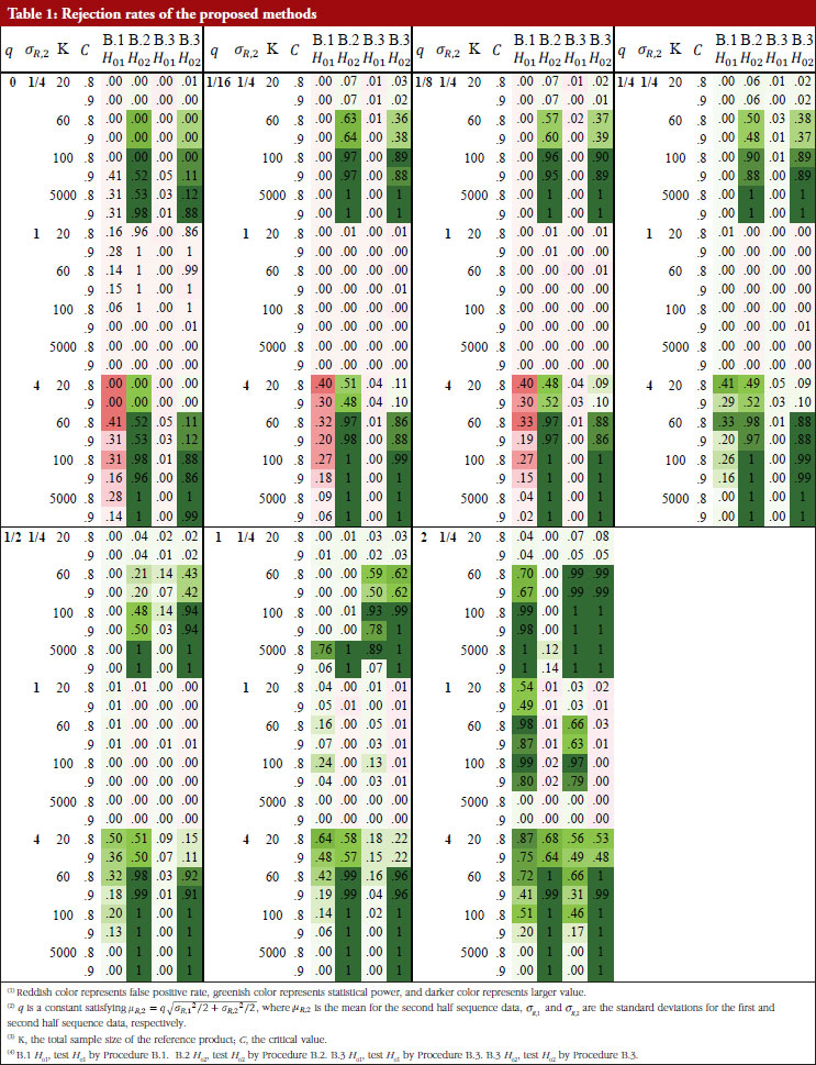
The true positive rate (power) of testing H01 by Procedure B.1 and B.3 is similar but lower when | µ R,2 – µ R,1|≥ σR/2 (i.e. the mean difference is not substantial) and  . When | µ R,2 – µ R,1| = σ R and , the power of H01 by Procedure B.3 is higher than with the use of B.1, and the power of H01 by Procedure B.3 is at medium (~0.40) or higher, if the sample size is small. When | µ R,2 – µ R,1| = 2 σR and K ≤ 60, the power of H01 by Procedure B.3 is adequate (~0.60 or higher).
The power of testing H02 by Procedure B.2 is higher than with the use of B.3 when | µ R,2 – µ R,1| ≥ σR/2: the power of both testing H02 in B.2 and B.3 is substantial (~0.90) when K ≤ 1000 given σ R,2/ σ R,1 = 1/4 or 4, and is substantial (~0.90) when K = 5,000 given σ R,2/ σ R,1 = 1/2 or 2. When | µ R,2 – µ R,1| = σ R the power of testing H02 by Procedure B.3 is higher than that using Procedure B.2 with the following observations: the power of testing H02 by Procedure B.3 is always adequate (~0.60) when K ≤ 60 gvien σ R,2/ σ R,1 = 1/4 or 4. When | µ R,2 – µ R,1| = 2 σ 2, the power of testing H02 is substantial (~0.90) when K ≤ 60 given σ R,2/ σ R,1 = 1/4 or 4 and the power is adequate (~0.60) when K ≤ 60 given σ R,2/ σ R,1 = 1/4 or 4.
The results show that when the sample size is limited; a common situation in practice for biosimilar studies, the power of testing drift in mean/variability is inadequate when the underlying true parameter configuration deviates slightly from the null hypothesis. But when the deviation is substantial, the proposed procedures still have adequate power even with a limited sample size.
An example
For illustrative purpose, consider an example concerning analytical similarity assessment of a Herceptin (trastuzumab) biosimilar regulatory submission. Trastuzumab (Herceptin®) is a monoclonal antibody, that contains human framework regions combined with complementarity-determining regions of a murine antibody that binds to human epidermal growth factor receptor 2 (HER2). Herceptin® was approved by FDA (September 1998) and European Medicines Agency (August 2000) for use in treating certain breast cancers that overexpress HER2. Herceptin®-containing regimens are the standard of care for the treatment of HER2-positive breast cancers, providing significant clinical benefit in adjuvant settings against early as well as advanced or metastatic breast cancers [21].
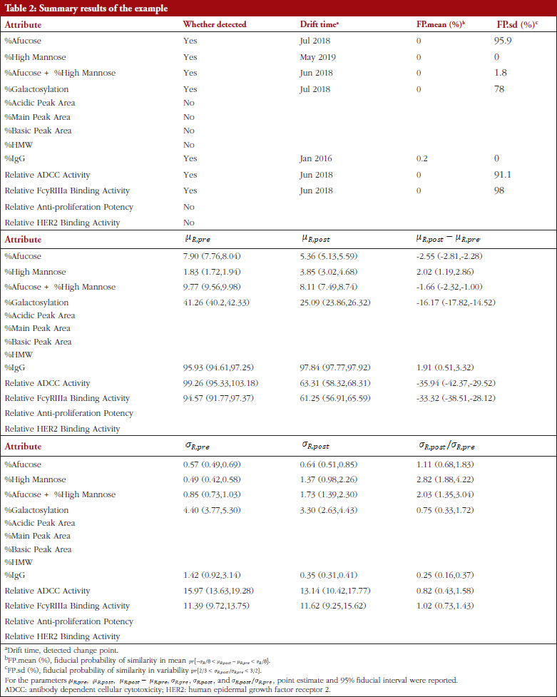
For the development of a biosimilar version of trastuzumab, the reference product (Herceptin®) was extensively characterized for the main physicochemical and biological properties by standard or state-of-the-art analytical methods, using up to 103 unexpired lots in total of EU and US Herceptin® lots expiring between March 2015 and December 2019 [7]. The data used here are shown in Figure 1 as scatter plots of attribute value versus expiry date for thirteen attributes. As indicated by Kim et al. [7], a high degree of consistency was observed for all the tested properties for lots with expiry dates up to July 2018. However, among the lots expiring in August 2018 or later, a downward drift was observed in %afucose. Furthermore, the upward drift of %high mannose was observed in the lots with expiry dates from June 2019 to December 2019. As a result, the combination of %afucose and %high mannose showed two marked drifts in the lots with expiry dates from August 2018 to December 2019, which was supported by the similar trend of biological data, such as FcgRIIIa binding and ADCC activity. Considering that ADCC is one of the clinically relevant mechanisms of action for trastuzumab, the levels of %afucose and %high mannose should be tightly monitored as critical quality attributes for biosimilar development of trastuzumab.
However, Kim et al. [7] determined the drift time points by observing the scatter plots without statistical rigour. Such a subjective judgement would lead to controversial conclusions when different researchers make different judgements. Besides, Kim et al. only determined drifts in mean (location) without considering drifts in variance, although their reported figures indicate potential variance drifts for some attributes. As discussed in the previous sections, the drifts could be due to: (i) drift in mean; (ii) drift in variability; or (iii) drift in both mean and variability. For detecting possible drift in mean, drift in variability, or drift in both mean and variability, the proposed Procedure B.3 with the critical value C = 0.95 was performed to validate the observed drifts as described by Kim et al. [7]. The raw data of thirteen attributes was extracted by digitizing the figures reported by Kim et al. [7], with the help of a tool ‘WebPlotDigitizer’ (https://automeris.io/WebPlotDigitizer/). Then Procedure B.3 was applied to detect and test drift in mean/variance for each attribute with similarity assumptions.
Table 2 shows the summary results using Procedure B.3 for detecting and testing drift in mean/variance of the thirteen attributes. Four attributes, %Afucose, %Galactosylation, Relative ADCC Activity and Relative FcyRIIIa Binding Activity, were detected to have a drift in mean around July 2018. Three attributes, %High Mannose, %Afucose + %High Mannose and %IgG, were detected to have drifts in both mean and variance around May 2019, Jun 2018 and Jan 2016, respectively. There were no drifts detected by our procedure for the remaining attributes. Figure 1 presents the data with all detected drift for each attribute. While for most attributes similar conclusions with respect to mean drift were reached to the results reported by Kim et al. [7], the proposed procedure further detected a mean drift of %IgG that occurred around January 2016. Moreover, a drift in variance for three attributes was detected that could provide important new information for assessing the standard deviation of the reference product while implementing an equivalence test of CQAs.
Discussion
When performing analytical similarity assessment on certain critical quality attributes (CQAs) that are relevant to clinical outcomes, a potential drift in mean response and/or drift in variability associated with the response of the reference product over time may be observed. When there is drift in the reference product over time, concern exists that the lots before and after the drift may not be biosimilar themselves. In this case, it is of particular importance to regulators and sponsors regarding which lots (i.e. reference lots before the drift, after the drift, or combined) should be used for a valid, accurate and reliable analytical similarity assessments.
In this article, three combined procedures incorporating several statistical tests for the detection of possible drift in mean, drift in variability, and drifts in both mean and variability are presented. If a notable drift in mean and/or variability are observed, it is of interest to estimate at which time the drift occurred and validate the drift using the proposed statistical tests. The information generated by the tests proposed provides valuable information for making decisions regarding which lots should be included in analytical similarity assessments. The inherent properties of biological therapeutics make them highly sensitive to changes in manufacturing conditions. Because of their high structural complexity compared with small molecules, even minor alterations (e.g. pH, temperature and manufacturing site) may reduce product consistency and cause drifts in target attributes [8]. Therefore, in practice, drifts in either mean, variability, or both inevitably occur, potentially due to laboratory test procedures and/or manufacturing process changes. When there is a significant drift in mean, variability, or both, the lots before and after the drift are not biosimilars. Therefore, it is suggested that regulatory guidance regarding the detection and assessment of any such post-approval changes should be developed.
Depending on specific situations, other distributions may be more appropriate to use rather than a normal distribution. The proposed approach can be easily extended to accommodate different distribution types, such as Exponential, Gamma, and Poisson distributions, for which change point detection methods and software are also well developed [18]. Note that Kim et al. [7] determined two drifts by their observations of the scatter plots for some attributes. In practice, multiple change points may occur and be detected. Under such situations, one may account for multiple hypotheses testing of similarity in mean/variance between more than two sub-datasets determined by the detected change points. For example, three testings given two detected change points and six testings given three detected change points have been performed using the methods described here. Accordingly, the proposed methods can be readily generalized to allow for multiple testing, for instance, by simply using 1 – (1 – C)/ Q instead of C and applying a Bonferroni correction where Q is the number of testings.
Though the proposed statistical test may be used for detecting drifts in biosimilar studies, one of its drawbacks is it may be unable to maintain the desired true positive rate under some special circumstances as illustrated in Table 1. There are some potential methods might alleviate this problem. For example, the segmented regression model has been wildly used in assessing the impact of intervention in time series studies by analysing changes in intercept and slope [22, 23]. Though segmented regression can be used to detect drifts in the distribution of time series data, it has seldom been used for drift detection for biosimilar products.
Conclusion
In summary, a statistical method is proposed that performs well to detect drift in the mean/variability of biological products while controlling false positive rates and maintaining true positive rates even when the number of lots tested is large.
Acknowledgement
There is no other contributor to this manuscript that is not listed in the author list. There is no funding information and prior presentations.
Competing interests: None.
Provenance and peer review: Not commissioned; externally peer reviewed.
Authors
Jiayin Zheng1, PhD
Peijin Wang2, MS
Yixin Wang3, PhD
Shein-Chung Chow2, PhD
1Division of Public Health Sciences, Fred Hutchinson Cancer Center, Seattle, Washington, USA
2Duke University School of Medicine, Durham, North Carolina, USA
3Vaccine and Infectious Disease Division, Fred Hutchinson Cancer Center, Seattle, Washington, USA
References
1. U.S. Food and Drug Administration. Guidance document. Scientific considerations in demonstrating biosimilarity to a reference product. 2015 [homepage on the Internet]. [cited 2023 Jan 3]. Available from: https://www.fda.gov/regulatory-information/search-fda-guidance-documents/scientific-considerations-demonstrating-biosimilarity-reference-product
2. U.S. Food and Drug Administration. FDA withdraws draft guidance for industry. Statistical approaches to evaluate analytical similarity. 2017 [homepage on the Internet]. [cited 2023 Jan 3]. Available from: https://www.fda.gov/drugs/drug-safety-and-availability/fda-withdraws-draft-guidance-industry-statistical-approaches-evaluate-analytical-similarity
3. U.S. Food and Drug Administration. Guidance document. Development of therapeutic protein biosimilars: comparative analytical assessment and other quality-related considerations. 2019 [homepage on the Internet]. [cited 2023 Jan 3]. Available from: https://www.fda.gov/regulatory-information/search-fda-guidance-documents/development-therapeutic-protein-biosimilars-comparative-analytical-assessment-and-other-quality
4. Son S, Oh M, Choo M, Chow SC, Lee SJ. Some thoughts on the QR method for analytical similarity evaluation. J Biopharm Stat. 2020;30(3):521-36.
5. Vulto AG, Jaquez OA. The process defines the product: what really matters in biosimilar design and production? Rheumatology (Oxford). 2017; 56(suppl_4):iv14-iv29.
6. Schiestl M, Stangler T, Torella C, Cepeljnik T, Toll H, Grau R. Acceptable changes in quality attributes of glycosylated biopharmaceuticals. Nat Biotechnol. 2011;29(4):310-2.
7. Kim S, Song J, Park S, Ham S, Paek K, Kang M, et al. Drifts in ADCC-related quality attributes of Herceptin®: impact on development of a trastuzumab biosimilar. MAbs. 2017;9(4):704-14.
8. Ramanan S, Grampp G. Drift, evolution, and divergence in biologics and biosimilars manufacturing. BioDrugs. 2014;28(4):363-72.
9. Schneider, CK. Biosimilars in rheumatology: the wind of change. Ann Rheum Dis. 2013;72(3):315-8.
10. JMP. Quality and reliability methods. JMP Version 10.1, A Business Unit of SAS, SAS Campus Drive, Cary, NC 27513. 2012.
11. Salah S, Chow SC, Song F. On the evaluation of reliability, repeatability, and reproducibility of instrumental evaluation methods and measurement systems. J Biopharm Stat. 2017;27(2):331-7.
12. Truong C, Oudre L, Vayatis N. Selective review of offline change point detection methods. Signal Processing. 2020;167:107299.
13. Niu YS, Hao N, Zhang H. Multiple change-point detection: a selective overview. Stat Sci. 2016;31(4):611-23.
14. Fisher RA. The fiducial argument in statistical inference. Ann Eugen. 1935;6(4):391-8.
15. Zheng J, Chow SC, Yuan M. On assessing bioequivalence and interchangeability between generics based on indirect comparisons. Stat Med. 2017;36(19):2978-93.
16. Page ES. Continuous inspection schemes. Biometrika. 1954;41(1/2):100-15.
17. Page ES. A test for a change in a parameter occurring at an unknown point. Biometrika. 1955;42(3/4):523-7.
18. Killick R, Fearnhead P, Eckley IA. Optimal detection of changepoints with a linear computational cost. J Am Stat Assoc. 2012;107(500):1590-8.
19. Killick R, Eckley I. changepoint: An R package for changepoint analysis. J Stat Softw. 2014;58(3):1-19.
20. Holm S. A simple sequentially rejective multiple test procedure. Scand J Statist. 1979;65-70.
21. Pivot X, Curtit E, Lee YJ, Golor G, Gauliard A, Shin D, et al. A randomized phase I pharmacokinetic study comparing biosimilar candidate SB3 and trastuzumab in healthy male subjects. ClinTher. 2016;38(7):1665-73.
22. Taljaard M, McKenzie JE, Ramsay CR, Grimshaw JM. The use of segmented regression in analysing interrupted time series studies: an example in pre-hospital ambulance care. Implement Sci. 2014;9:77
23. Quintens C, Coenen M, Declercq P, Casteels M, Peetermans WE, Spriet I. From basic to advanced computerised intravenous to oral switch for paracetamol and antibiotics: an interrupted time series analysis. BMJ Open. 2022;12(4):e053010.
|
Author for correspondence: Peijin Wang, MS, Department of Biostatistics and Bioinformatics, Duke University School of Medicine, 2424 Erwin Road, 11017 Hock Plaza, Durham NC 27705, USA |
Disclosure of Conflict of Interest Statement is available upon request.
Copyright © 2023 Pro Pharma Communications International
Permission granted to reproduce for personal and non-commercial use only. All other reproduction, copy or reprinting of all or part of any ‘Content’ found on this website is strictly prohibited without the prior consent of the publisher. Contact the publisher to obtain permission before redistributing.